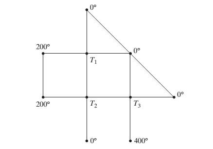
In a grid of wires, the temperature at exterior meshpoints is maintained at constant values (in °C), as shownin the accompanying figure. When the grid is in thermalequilibrium, the temperature T at each interior meshpoint is the average of the temperatures at the fouradjacent points. For example, T 2 = T 3 + T 1 + 200 + 0 4 . Find the temperatures T 1 , T 2 , and T 3 when the grid isin thermal equilibrium.
In a grid of wires, the temperature at exterior meshpoints is maintained at constant values (in °C), as shownin the accompanying figure. When the grid is in thermalequilibrium, the temperature T at each interior meshpoint is the average of the temperatures at the fouradjacent points. For example, T 2 = T 3 + T 1 + 200 + 0 4 . Find the temperatures T 1 , T 2 , and T 3 when the grid isin thermal equilibrium.
In a grid of wires, the temperature at exterior meshpoints is maintained at constant values (in °C), as shownin the accompanying figure. When the grid is in thermalequilibrium, the temperature T at each interior meshpoint is the average of the temperatures at the fouradjacent points. For example,
T
2
=
T
3
+
T
1
+
200
+
0
4
. Find the temperatures
T
1
,
T
2
,
and
T
3
when the grid isin thermal equilibrium.
A cup of water at an initial temperature of 81°C is placed in a room at a constant temperature of 24°C. The temperature of the water is measured every 5 minutes during a half-hour period. The results are recorded as ordered pairs of the form (t, T), where t is the time (in minutes) and T is the temperature (in degrees Celsius).
(0, 81.0°), (5, 69.0°), (10, 60.5°), (15, 54.2°), (20, 49.3°), (25, 45.4°), (30, 42.6°)
(a) Subtract the room temperature from each of the temperatures in the ordered pairs. Use a graphing utility to plot the data points (t, T) and (t, T − 24).
(b) An exponential model for the data (t, T − 24) is T − 24 = 54.4(0.964)t. Solve for T and graph the model. Compare the result with the plot of the original data.
(c) Use a graphing utility to plot the points (t, ln(T − 24)) and observe that the points appear to be linear.
Use the regression feature of the graphing utility to fit a line to these data. This resulting line has the form ln(T − 24) = at + b, which is…
An engineer wants to determine the spring constant for a particular spring. She hangs
various weights on one end of the spring and measures the length of the spring each time. A
scatterplot of length (y) versus load (x) is depicted in the following figure.
Inad
a Is the model y = P, +B, x an empirical model or a physical law?
b.
Should she transform the variables to try to make the relationship more linear, or
would it be better to redo the experiment? Explain.
In your Capstone software create a table with the following variables:
Position x, m: 1, 2, 3, 4
Coefficient of friction μ: 0.36
Velocity v, m/s: v=V 2. u.9.8.x
Need a deep-dive on the concept behind this application? Look no further. Learn more about this topic, algebra and related others by exploring similar questions and additional content below.


 Algebra: Structure And Method, Book 1AlgebraISBN:9780395977224Author:Richard G. Brown, Mary P. Dolciani, Robert H. Sorgenfrey, William L. ColePublisher:McDougal Littell
 Algebra & Trigonometry with Analytic GeometryAlgebraISBN:9781133382119Author:SwokowskiPublisher:Cengage